
When working with massive Excel spreadsheets, evaluating the info from two columns will be time-consuming. As an alternative of analyzing the columns and writing “Match” or “Mismatch” right into a separate column, you should utilize Excel’s capabilities to streamline the method.
We’ll check out learn how to use totally different Excel capabilities to match two columns and determine matching or mismatching knowledge.
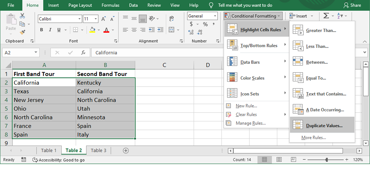
1. The way to Spotlight Duplicate Information
If you wish to evaluate two columns in Excel, however don’t wish to add a 3rd column exhibiting if the info exists in each columns, you should utilize the Conditional Formatting function.
- Choose the info cells you wish to evaluate.
- Head to the Dwelling tab.
- From the Types group, open the Conditional Formatting menu.
- Click on Spotlight Cells Guidelines > Duplicate Values.
- Within the Duplicate Values window, be certain that the Format cells that comprise choice is ready to Duplicate and select the formatting choice subsequent to values with.
- Click on OK.
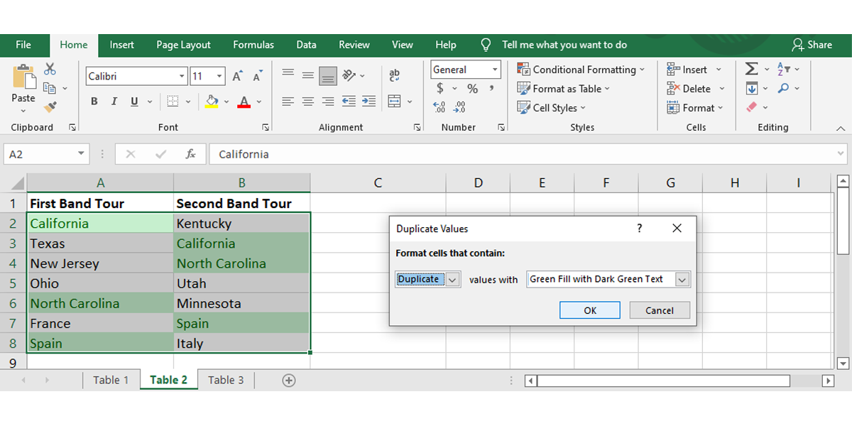
Excel will now spotlight the names which are current in each columns.
2. The way to Spotlight Distinctive Information
You should utilize the identical perform if you wish to determine knowledge that isn’t a part of each columns.
- Choose the info set.
- As soon as once more, head to Dwelling > Conditional Formatting > Spotlight Cells Guidelines > Duplicate Values.
- For Format cells that comprise, select Distinctive.
- Choose how the mismatched knowledge ought to be highlighted and click on OK.
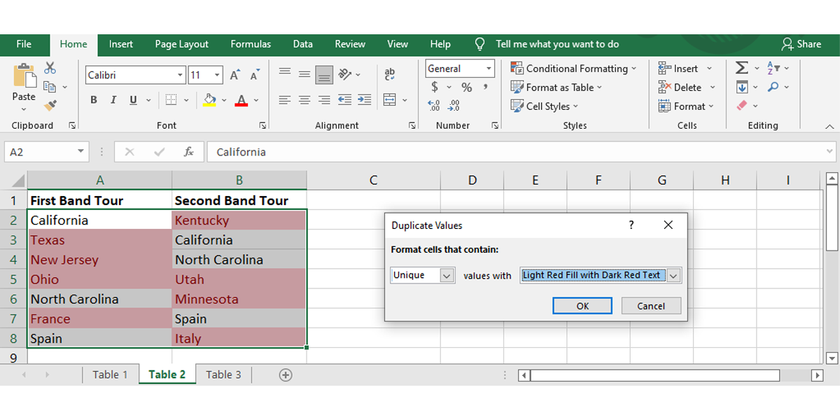
Excel will now spotlight the names that may be discovered solely in one of many two columns.
Whereas these strategies are fairly straightforward to make use of, they won’t be environment friendly for bigger spreadsheets. So we’ll check out extra complicated options that present you which of them rows have the identical knowledge or use an extra column to show values indicating if the info matches or not.
3. Spotlight Rows With Equivalent Information
In the event you want a greater visible illustration of equivalent knowledge, you can also make Excel discover matching values in two columns and spotlight the rows with matching knowledge. As we did on the earlier technique, we’ll use the Conditional Formatting function, however will add a number of additional steps.
This manner, you should have a visible indicator that can provide help to determine matching knowledge sooner than studying by means of a separate column.
Comply with these steps to make use of Excel’s conditional formatting to match two units of information:
- Choose the info you wish to evaluate (don’t embrace the headers) and open the Dwelling tab.
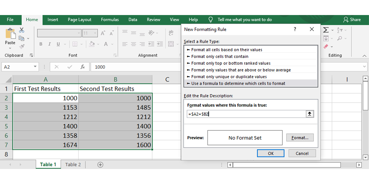
- Click on Conditional Formatting and choose New Rule.
- From Choose a Rule Kind, click on Use a method to find out which cells to format.
- Enter =$A2=$B2 into the sector beneath Format values the place this method is true. Right here, A and B correspond to the 2 columns we’re evaluating.
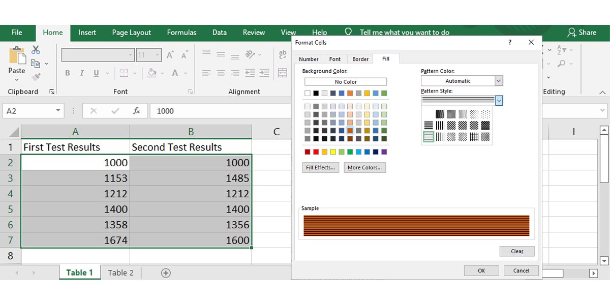
- To customise how Excel will spotlight the rows, click on Format and within the Format cells window, choose the Fill tab. You may select the background colour, sample type, and sample colour. You’re going to get a pattern, so you’ll be able to preview the design. Click on OK when you’ve accomplished the customization course of.
- Click on OK within the New Formatting Rule window, so Excel will spotlight the rows with matching knowledge immediately.
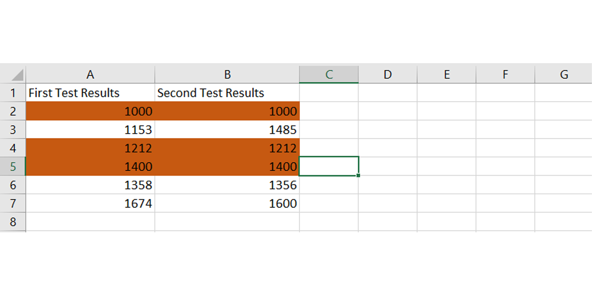
When evaluating two columns in Excel utilizing this technique, you may as well spotlight the rows with totally different knowledge. Undergo the above steps and at step 5, enter the =$A2<>$B2 method throughout the Format values the place this method is true discipline.
4. Establish Matches With TRUE or FALSE
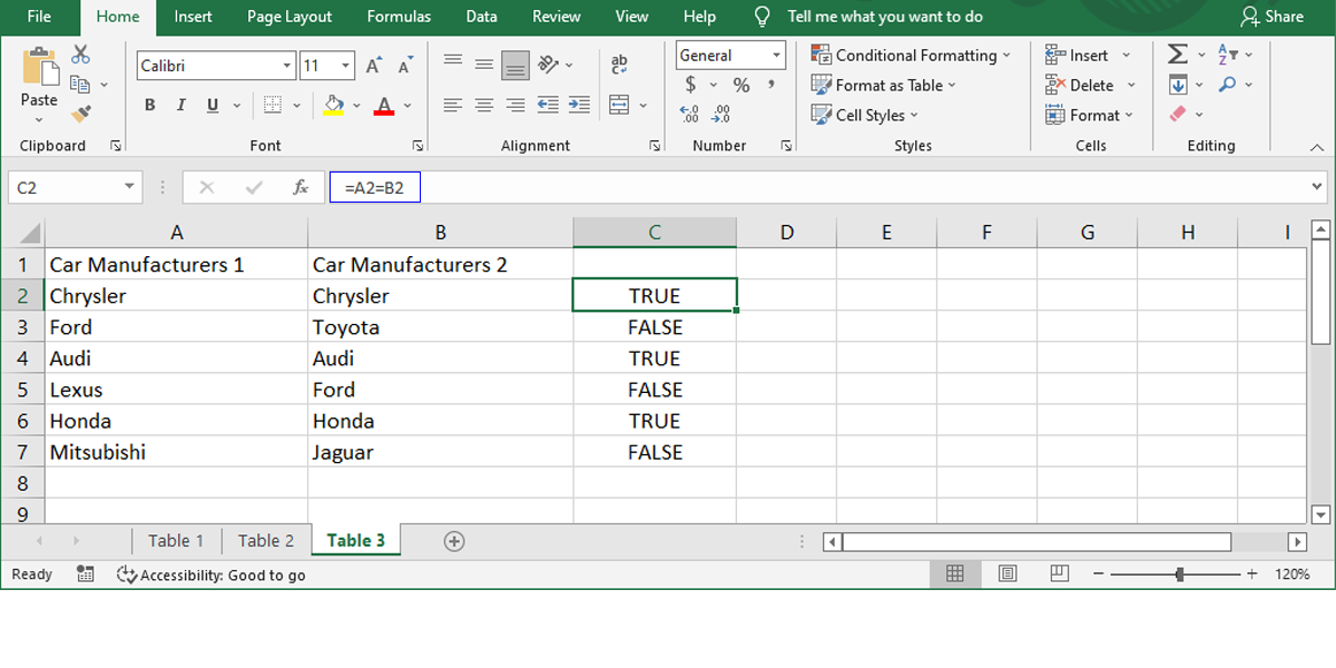
You may add a brand new column when evaluating two Excel columns. Utilizing this technique, you’ll add a 3rd column that can show TRUE if the info matches and FALSE if the info doesn’t match.
For the third column, use the =A2=B2 method to match the primary two columns. In the event you assume your spreadsheet will look too crowded with the TRUE and FALSE rows, you’ll be able to set a filter in Excel, so it’ll solely present the TRUE values.
5. Examine Two Columns With an IF Perform
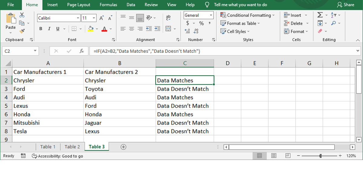
A distinct technique to investigate Excel knowledge from two columns is to make use of an IF perform. That is much like the above technique, but it surely comes with the benefit you could customise the displayed worth.
As an alternative of getting the TRUE or FALSE values, you’ll be able to set the worth for matching or totally different knowledge. For this instance, we’ll use the Information matches and Information doesn’t match values.
The method we’ll use for the column exhibiting the outcomes is =IF(A2=B2,”Information Matches”,”Information Doesn’t Match”).
6. Examine Two Columns With a VLOOKUP Perform and Discover Matching Information
One other method to have Excel discover duplicates in two columns is to make use of a VLOOKUP perform. Excel will evaluate every cell within the second column towards the cells within the first column.
Use the =VLOOKUP(B2,$A$2:$A$14,1,0) for the column displaying the outcomes. Simply be sure to alter the info vary.
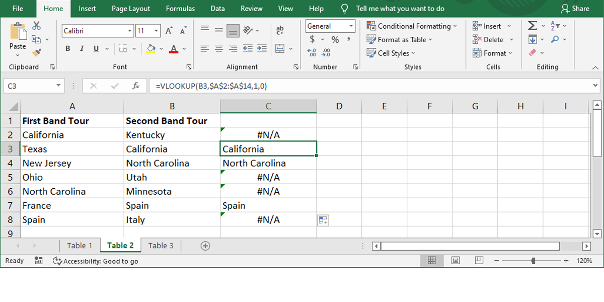
When utilizing this method, Excel will show the matching knowledge or use a #N/A price. Nevertheless, the #N/A worth is perhaps complicated, particularly when you ship the spreadsheet to another person. If they aren’t skilled with regards to Excel, they may imagine there’s a mistake.
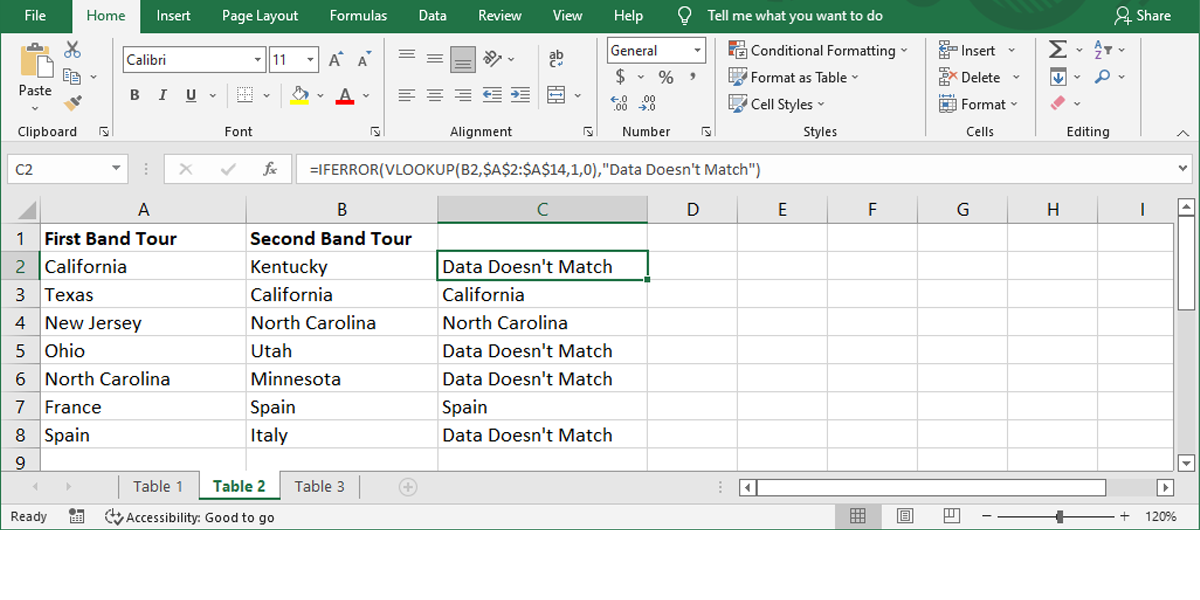
So to keep away from any confusion, improve the VLOOKUP perform to an IFERROR perform. If you should discover knowledge that’s in column B and can also be in column A, use the =IFERROR(VLOOKUP(B2,$A$2:$A$14,1,0),”Information Does not Match”) method.
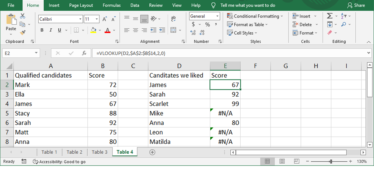
7. The way to Examine Two Columns and Extract Information
Moreover evaluating two Excel columns for matches, you may as well use the VLOOKUP perform to extract matching knowledge. This can prevent time as you don’t must manually undergo the primary column and seek for related knowledge.
Additionally, if knowledge within the second column misses from the primary column, Excel will show a #N/A price. For this, use the =VLOOKUP(D2,$A$2:$B$14,2,0) method.
Word: If you wish to shield your outcomes towards spelling errors, use the =VLOOKUP(“*”&D2&”*”,$A$2:$B$14,2,0) method. Right here, the asterisk (*) has the position of a wild card character, changing any variety of characters.
Examine Information With Ease
As we’ve mentioned, there are many methods and methods you should utilize to match two columns in an Excel spreadsheet and get the perfect outcomes. And Excel has much more instruments that may provide help to keep away from repetitive duties and prevent lots of time.
Learn Subsequent
About The Creator
