Formatting data in Microsoft Excel can be tricky, especially when you need to amend a large dataset already filled out. Numbering the rows in Excel is an example of such formatting.
If a dataset is small and continuous, one can easily number its rows manually or by auto-filling sequence. When the dataset is large and inconsistent, some data needs to be added or removed from the middle, or when you need to filter the data in a specific column, the numbering gets messed up.
Let’s explore different ways to number rows of the consistent and inconsistent (empty rows) datasets in Microsoft Excel.
1. Numbering Rows of a Consistent Dataset in Excel Using Fill Handle and Fill Series:
Using the Fill Handle or Fill Series is the easiest way to number rows when you have a consistent dataset with no empty rows.
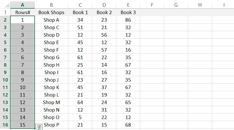
For better understanding, let’s apply both ways of numbering rows to a dataset shown below:
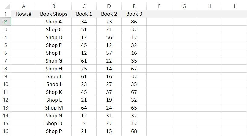
To number rows with Fill Handle, follow these steps:
- Put 1, 2, and 3 in cells A2, A3, and A4.
- Select the cells A2 through A4.
- A plus icon will appear in the bottom-right corner of the last selected cell when your cursor hovers over it.
- Clicking twice on it will number all the continuous rows below it.
Therefore, if no empty rows appear throughout the dataset, it is a fast method for numbering rows. However, Fill Handle does not work in these two cases:
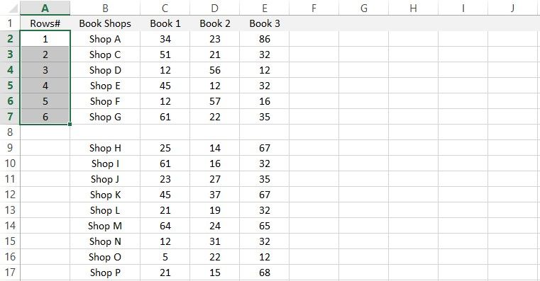
- Whenever the Fill Handle encounters an inconsistency (an empty row), it will automatically stop.
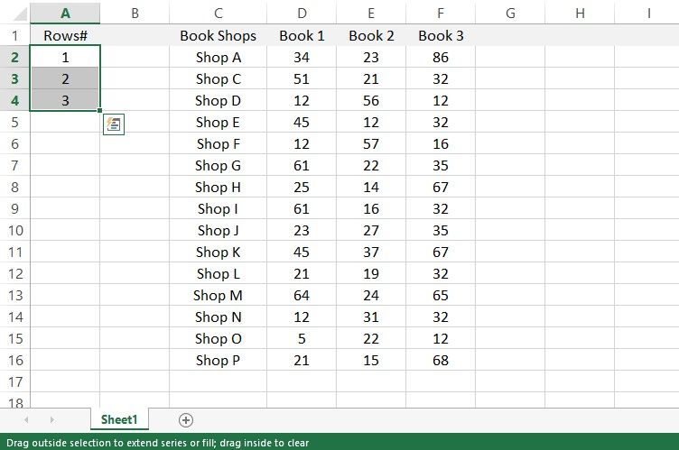
- If the adjacent column where you are using Fill Handle is empty, it won’t work.
However, there is a workaround to this, namely manual auto-filling of the sequence. In this way, even if there is an inconsistency in the dataset or the adjacent column is empty, you can still number the rows all the way to the end.
Auto-filling is as simple as dragging the lower-right corner of selected cells where the plus sign is displayed and extending it to the end.
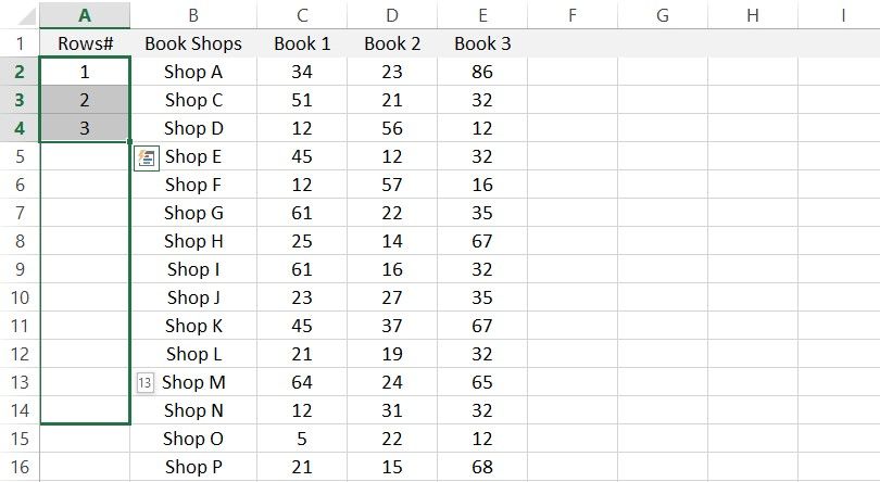
But this method is not viable due to the following reasons:
- It also numbers any empty rows that come in its way, which of course, we do not want.
- Manually dragging a dataset to the bottom becomes problematic if the dataset is extensive.
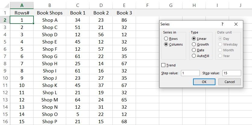
Alternatively, you can use the Fill Series method if you do not want to manually drag sequences in a large dataset but still want auto-fill data to the end. Let’s look at how it works.
- Note the total number of filled rows in the dataset by pressing CTRL + End.
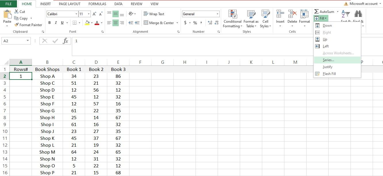
- In cell A2, enter 1.
- Select Series from the Fill dropdown in the Editing section of the Home tab.
- Choose Columns in Series in and Linear in Type.
- Set Stop value to the total number of filled rows and Step value to 1.
- Click OK.
The rows will be automatically numbered up to the last filled one, including the empty ones. Although it eliminates manual dragging and does not stop filling at the empty row, it won’t work when making professional spreadsheets since it numbers empty rows, which we don’t want.
Furthermore, since both methods are static, if you delete a row and move or replace it, you will have to renumber it. Nevertheless, both methods are easy to use and work well when the data is consistent.
Let’s look at how to number inconsistent datasets with empty rows using the COUNTA and IF functions.
2. Using COUNTA and IF Functions to Number Rows in an Inconsistent Dataset
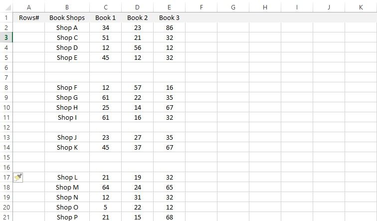
The COUNTA function skips empty rows while numbering the filled ones in sequence. To see how it works, let’s apply it to an inconsistent dataset:
- Consider the following dataset:
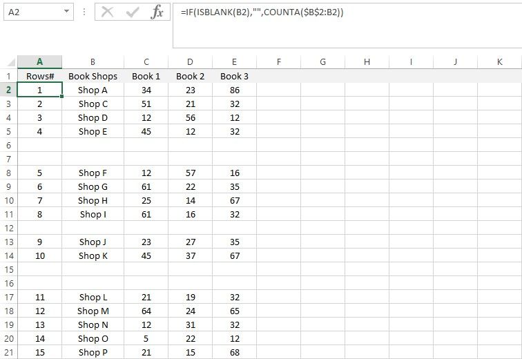
- Fill in the following formula in cell A2:
=IF(ISBLANK(B2),"",COUNTA($B$2:B2))
- Using auto-fill, fill in the remaining cells below.
You can see that it skipped over the empty cells while numbered only the filled ones in order. Here, the IF function decides whether the adjacent cell is empty. It leaves the rows empty if adjacent cells are empty and count them if they are filled.
Moreover, this method of numbering rows is dynamic, so when you add, replace, or remove a row, the numbering will automatically be updated.
However, what if you need to fill the dataset and want to maintain the row numbers? In this case, the combination of IF and COUNTA won’t help, and neither will Fill Handle or Fill Series.
Then you can go for another approach, using the SUBTOTAL function to maintain row numbering in the datasheet while filtering data.
3. Using SUBTOTAL Function
Let’s view the SUBTOTAL function syntax before we apply it to the dataset.
=SUBTOTAL(function_num, range 1, [range 2..])
Range 1 indicates the range of the dataset where the function is to be applied. The function_num indicates where your desired function is located in the list, as shown below.
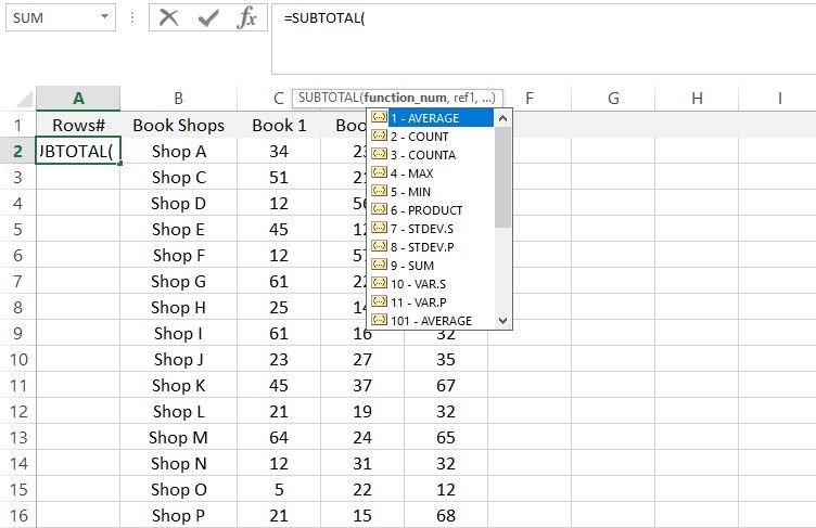
To number rows using SUBTOTAL, follow these steps:
- Go to cell A2.
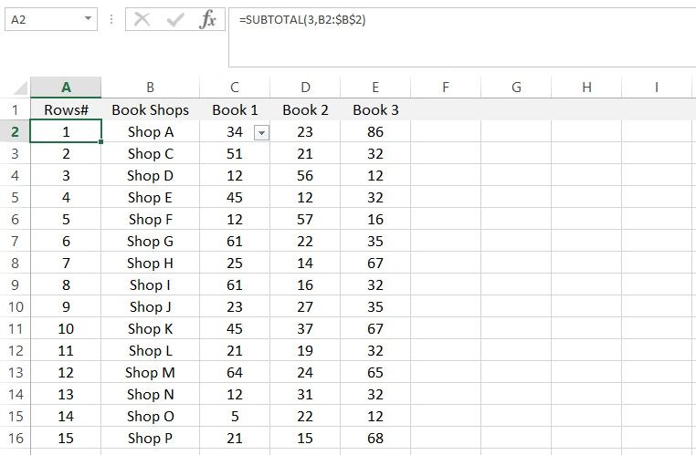
- There, enter the following formula:
=SUBTOTAL(3,B2:$B$2)
- Fill in the sequence to populate entries in the cells below.
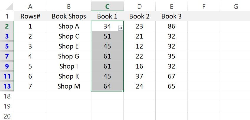
Now, as shown below, when you filter the data in any other column, the row numbering will change automatically in the correct order.
Comparing the Uses of Each Method
Let’s briefly review where all three methods are useful:
- As long as you have consistent data with no empty rows, you can use Fill Handle or Fill Series to number the rows.
- If the data is inconsistent, and you only need to number the rows (without filtering them later), you can use the second method of combining the COUNTA function with an IF function.
- The SUBTOTAL function will work whenever you need to filter data while maintaining row numbering.
Number Rows With Ease in Microsoft Excel
This way, no matter if the data is consistent or not, you can easily number the rows. Choose whichever method best suits your needs.
Besides these three methods, you can also use the ROW function and create an Excel table to number rows, but each of these approaches has its limitations.
Is it always a struggle to manage multiple worksheets with endless rows and columns? You can easily group rows and columns, so the data is easier for you to handle and easier for your clients and colleagues to navigate. Use them in your spreadsheets to make them look more professional.
Read Next
About The Author
